DendroNN, or the Resurrection of the Tree Classification Project

TreeID Dataset

Collecting and processing the tree data was a big learning experience. That’s the encouraging, optimistic way of saying that I made a ton of mistakes that I will never, ever repeat because I cringe at how obvious they feel in retrospect. This is still under active development and has attracted some outside interest, so you can follow along at the GitHub repo. So, what are we looking at here?

How was the data collected?

The beginning of this project was a collection of nearly 5,000 photos around my own neighborhood in Cleveland at the end of 2020. Not being an arborist, or even someone who leaves the house much, I hadn’t anticipated how difficult it would be to learn how to identify trees from just bark at the time. Because it was only of personal interest at the time, the project was put on ice.

At the end of 2022, I learned of a couple of helpful projects. The first and primary source of my data, the City of Pittsburgh paid for a tree inventory a few years ago. The species of tree, its GPS-tagged location, and other relevant data can be accessed as part of its Burghs Eye View program. It’s worth noting that Burghs Eye View isn’t just about trees, but is an admirable civic data resource in general. The second, and one which I unfortunately didn’t have time to use, is Falling Fruit, which has a bit of a different aim.

Using the Burghs Eye View map, I took a trip to Pittsburgh and systematically collected several thousand photos of tree bark using a normal smart phone camera. The procedure was simple:

  1. Start taking regularly spaced photos from the roots, less than a meter away from the tree bark, and track upward.
  2. When the phone it at arm’s reach, angle it upward to get one more shot of the canopy.
  3. Step to another angle of the tree and repeat, usually capturing about six angles of an adult tree.

Mistake 1 – Images too Large

Problem

The photos taken in Pittsburgh had a resolution of 3000×4000. An extremely common preprocessing technique in deep learning is scaling images down to, e.g. 224×224 or 384×384. Jeremy Howard in the Fast.ai course even plays with this, and developed a technique called progressive upscaling; images are scaled to 224×224, a model is trained on them, and then the model is trained on images that were scaled to a resolution more like 384×384.

I spent a lot of time trying to make this work, to the point where I started using cloud compute services to handle much larger images, to no avail. Ready to give up, I scoured my notebooks and noticed that some of the trees that the model was confusing more than the others looked very similar when scaled down to that size. It occurred to me that a lot of important fine details of bark was probably getting lost in that kind of compression. Okay, but so what?

Solution

Cutting the images up. I suspect this solution is somewhat specific to problems like this one. It doensn’t seem like it would be useful for classification purposes if you were to cut photos of fruit or houses into many much smaller patches. But tree bark is basically just a repeating texture. Even before realizing the next mistake, I noticed improvements by scaling down to 500×500 images, then finally a more drastic improvement by going down to 250×250.

In some ways this gave me a lot more data. If you follow the match, a 3000×4000 image becomes at most 192 usable 250×250 patches. I at first thought it was a little suspicious, but I looked around and doing it this way isn’t without precedent. There is a Kaggle competition for histopathological cancer detection where this technique comes up, for instance.

Mistake 2 – Too Much Extraneous Data

Problem

A non-trivial amount of this data got thrown out. At the time, I was working on the impression that the AI would need to take in as much data as it could. What I hadn’t considered was that some kinds of tree data, even some kinds of bark data, would be substantially more useful than others in classifying the trees. To borrow a data science idea, I hadn’t done a principle component analysis and wasted a lot of time. Many early training sessions were spent trying to get the model to classify trees based on images that included:

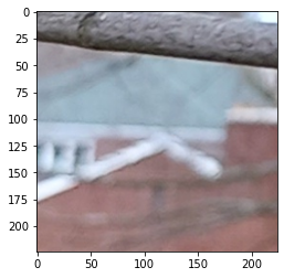
  • Roots and irregular branches
  • Soil and stray leaves
  • Tree canopy that wasn’t specific
  • Excessively blurry images
  • Tree bark that was covered in lichen or moss, damaged, diseased
  • Potentially useful, but at an angle or a distance that just got in the way

The end result was that it might require an inhumanly large dataset to achieve learning in any meaningful way. Early models could somewhat distinguish photos of oaks and pines in this way, but the results were too poor to be worth reporting.

Solution

Well, I ended up with two solutions.

The first was training a binary classifier to detect usable bark. The first time this came up, I was still working with the 500×500 patches, which worked out to just shy of 200,000 images. Not exactly a manual number, but I’ve never seen an ocean that I didn’t think I could boil. I spent an afternoon sorting 30,000 images, realized I had only sorted 30,000 images, and then realized I accidentally made a halfway decent training set for a binary classifer.

That classifier sorted the remainder of those images in under an hour.

The second solution was, unfortunately, quite a bit less dramatic. It involved simply going through the original photos, picking out the ones that basically weren’t platonic bark taken at about torso level, and just repeating the process of dividing them into patches and feeding those into the usable bart sorter.

So, what does it actually look like?

Alright, we’re getting into a little of the code. First, we need to import some standard libraries. I’ll do some explaining for the uninitiated.

pandas handles data manipulation, here mostly CSV files. If you’ve done any work with neural networks before, you might have seen images being loaded into folders, one per class. I personally prefer CSV files because they make it easier to include other relevant things besides just the specific class of the image. I’ll show you an example shortly.

matplotlib is a library for annotation and displaying charts.

numpy is a library for more easily handling matrix operations.

PIL is a library for processing images. It’s used here mostly for loading purposes, and we can see that because we are loading the Image class from it.

In [1]:
import pandas as pd
import matplotlib.pyplot as plt
import numpy as np
from PIL import Image

import os

Something that was really helpful was the use of confidence values. For every patch that the usable bark sorter classified, it also returned its confidence in the classification. Looking at the results, it had a strong inclination to reject perfectly usable bark, but it also wasn’t especially confident about those decisions. We can use that to our advantange by only taking bark that it was very confident about.

In [2]:
def confidence_threshold(df, thresh=0.9, below=True):
    if below==True:
        return df[df['confidence'] < thresh]
    else:
        return df[df['confidence'] > thresh]

Loading the Data

What these files will ultimately look like is still in flux. Today, I’ll be walking you through some older ones that still have basically what we need right now. First, we load the partitions that were accepted or rejected by the usable bark sorter. We also do a little cleanup of the DataFrame.

In [49]:
reject_file = "../torso_reject.csv"
accept_file = "../torso_accept.csv"

reject_df = pd.read_csv(reject_file, index_col=0)
accept_df = pd.read_csv(accept_file, index_col=0)

accept_df
Out[49]:
path confidence
0 dataset0/pittsburgh_torso-250×250/0001/2023010… 0.776984
1 dataset0/pittsburgh_torso-250×250/0001/2023010… 0.999994
2 dataset0/pittsburgh_torso-250×250/0001/2023010… 0.890233
3 dataset0/pittsburgh_torso-250×250/0001/2023010… 0.503523
4 dataset0/pittsburgh_torso-250×250/0001/2023010… 0.999959
108057 dataset0/pittsburgh_torso-250×250/0079/2023010… 0.998933
108058 dataset0/pittsburgh_torso-250×250/0079/2023010… 0.999988
108059 dataset0/pittsburgh_torso-250×250/0079/2023010… 0.998984
108060 dataset0/pittsburgh_torso-250×250/0079/2023010… 1.000000
108061 dataset0/pittsburgh_torso-250×250/0079/2023010… 0.999999

108062 rows × 2 columns

I accidentally goofed up when generating the files by accidentally leaving a redundant “.jpg” in a script. The files have since been renamed, but because we’re using older CSVs, we need to make a quick fix here. The below is just a quick helper function that pandas can use to map to each path in the DataFrame.

In [50]:
def fix_path(path):
    path_parts = path.split('/')
    
    # Change 'dataset0' to 'dataset'
    #fn[0] = "dataset"
    
    # Remove redundant '.jpg'
    fn = path_parts[-1]
    fn = fn.split('_')    
    fn[1] = fn[1].split('.')[0]
    fn = '_'.join(fn)
    path_parts[-1] = fn
    path_parts[0] = "../dataset"
    path_parts = '/'.join(path_parts)
    return path_parts
In [51]:
accept_df['path'] = accept_df['path'].map(lambda x: fix_path(x))
reject_df['path'] = reject_df['path'].map(lambda x: fix_path(x))

And just to make sure it actually worked okay:

In [52]:
accept_df['path'].iloc[0]
Out[52]:
'../dataset/pittsburgh_torso-250x250/0001/20230106_113732(0)_7_1.jpg'

Alright, so what’s this?

In [53]:
accept_df
Out[53]:
path confidence
0 ../dataset/pittsburgh_torso-250×250/0001/20230… 0.776984
1 ../dataset/pittsburgh_torso-250×250/0001/20230… 0.999994
2 ../dataset/pittsburgh_torso-250×250/0001/20230… 0.890233
3 ../dataset/pittsburgh_torso-250×250/0001/20230… 0.503523
4 ../dataset/pittsburgh_torso-250×250/0001/20230… 0.999959
108057 ../dataset/pittsburgh_torso-250×250/0079/20230… 0.998933
108058 ../dataset/pittsburgh_torso-250×250/0079/20230… 0.999988
108059 ../dataset/pittsburgh_torso-250×250/0079/20230… 0.998984
108060 ../dataset/pittsburgh_torso-250×250/0079/20230… 1.000000
108061 ../dataset/pittsburgh_torso-250×250/0079/20230… 0.999999

108062 rows × 2 columns

In [54]:
 reject_df
Out[54]:
path confidence
0 ../dataset/pittsburgh_torso-250×250/0001/20230… 1.000000
1 ../dataset/pittsburgh_torso-250×250/0001/20230… 0.999809
2 ../dataset/pittsburgh_torso-250×250/0001/20230… 0.999998
3 ../dataset/pittsburgh_torso-250×250/0001/20230… 0.997332
4 ../dataset/pittsburgh_torso-250×250/0001/20230… 0.999979
93149 ../dataset/pittsburgh_torso-250×250/0079/20230… 0.651545
93150 ../dataset/pittsburgh_torso-250×250/0079/20230… 0.999999
93151 ../dataset/pittsburgh_torso-250×250/0079/20230… 0.982236
93152 ../dataset/pittsburgh_torso-250×250/0079/20230… 0.991354
93153 ../dataset/pittsburgh_torso-250×250/0079/20230… 0.897549

93154 rows × 2 columns

Around 108K patches were accepted, and around 93K were rejected. Looking at the confidence column, we see that there are a few that the model is somewhat uncertain about some of these. Let’s take a look at that.

First, we need a couple more helper functions. This one opens an image, converts it to RGB, resizes it to something presentable, and converts it to a numpy array.

In [22]:
def image_reshape(path):
    image = Image.open(path).convert("RGB")
    image = image.resize((224, 224))
    image = np.asarray(image)
    return image

Next, it will be helpful to be able to see a few of these patches at once. This next function will get patches in batches of 16 and arranges them in a 4×4 grid with matplotlib.

In [23]:
def get_sample(path_list):
    print("Generating new sample")
    new_sample = np.random.choice(path_list, 16, replace=False)
    
    samples = []
    paths = []
    for image in new_sample:
        samples.append(image_reshape(image))
        paths.append(image)
    return samples, paths

get_sample() takes a list of paths, so let’s extract those from the DataFrame.

In [24]:
reject_paths = reject_df['path'].values.tolist()
accept_paths = accept_df['path'].values.tolist()
In [26]:
samples, paths = get_sample(reject_paths)
plt.imshow(samples[1])
Generating new sample
Out[26]:
<matplotlib.image.AxesImage at 0x7fb632dda470>

Okay, let’s see a whole grid of rejects!

In [27]:
def show_grid(sample):
    rows = 4
    cols = 4
    img_count = 0
    fix, axes = plt.subplots(nrows=rows, ncols=cols, figsize=(15,15))
    
    for i in range(rows):
        for j in range(cols):
            if img_count < len(sample):
                axes[i, j].imshow(sample[img_count])
                img_count += 1
In [28]:
def new_random_grid(path_list):
    sample, paths = get_sample(path_list)
    show_grid(sample)
    return sample, paths
In [30]:
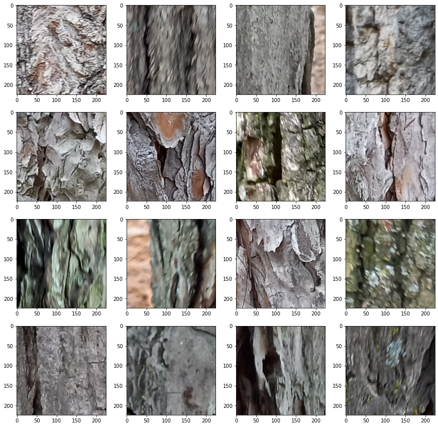
sample, paths = new_random_grid(reject_paths)
Generating new sample

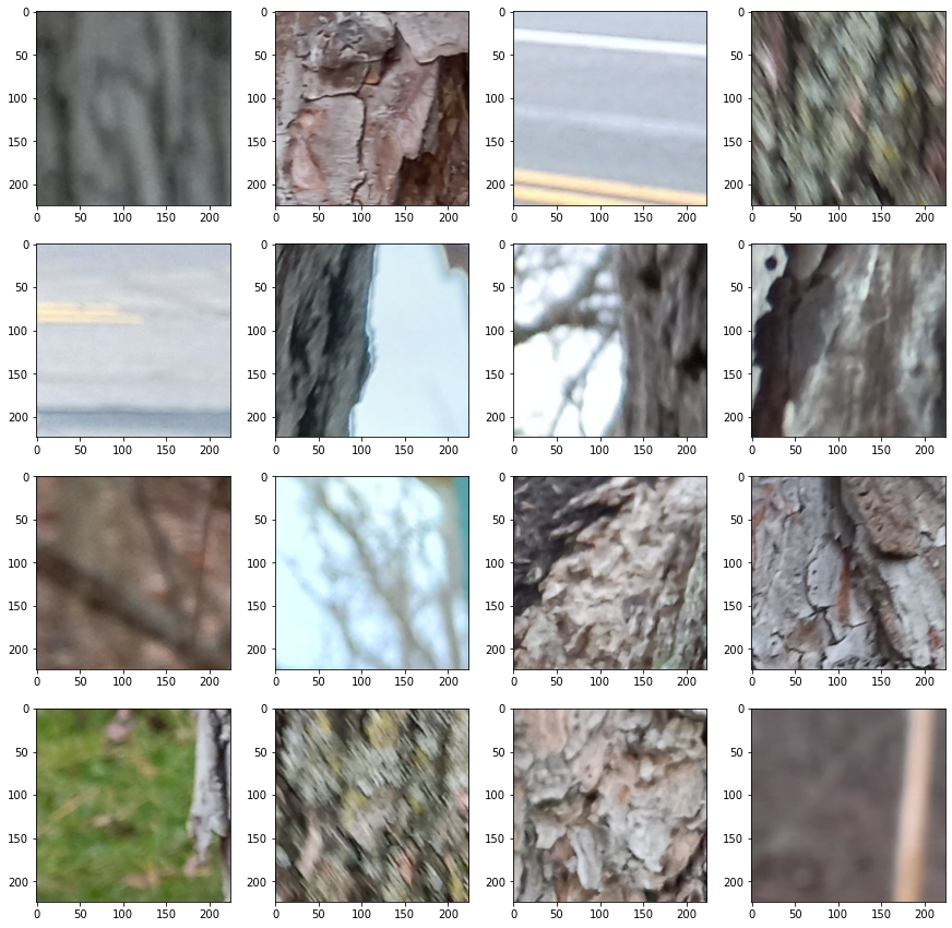
These are samples of the whole of the rejects list. I encourage you to run this cell a bunch of times if you’re following along at home. You should see a goodly number of things that aren’t remotely bark: bits of streets, signs, grass, dirt, and other stuff like that. You’ll also see a number of patches that are bark, but aren’t very good for training. Some bark is blurry, out of focus, or a part of the tree that I later learned wasn’t actually useful.

A fun thing to try is to see the stuff that the model rejected, but wasn’t very confident about.

In [35]:
reject_df_below_85 = confidence_threshold(reject_df, thresh=0.85, below=True)
reject_df_below_85_paths = reject_df_below_85['path'].values.tolist()
sample, paths = new_random_grid(reject_df_below_85_paths)
Generating new sample

Running this just once or twice usually reveals images that are a bit more… On the edge of acceptability. It’s not always clear why something got rejected. I haven’t ended up doing this yet, but something in the works is examining these low-confidence rejects in either training or, more likely, testing of the model. Mercifully, there is enough data that was unambiguously accepted that doing so hasn’t been a pressing need.

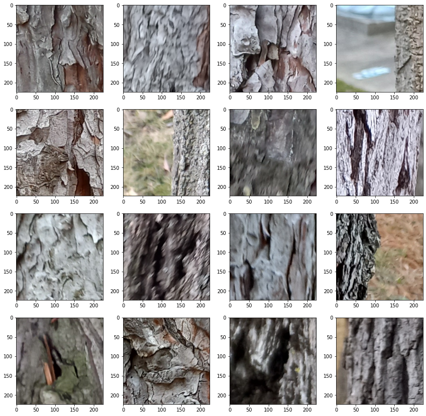
Speaking of, we should take a look at what got accepted, too.

In [39]:
sample, paths = new_random_grid(accept_paths)
Generating new sample

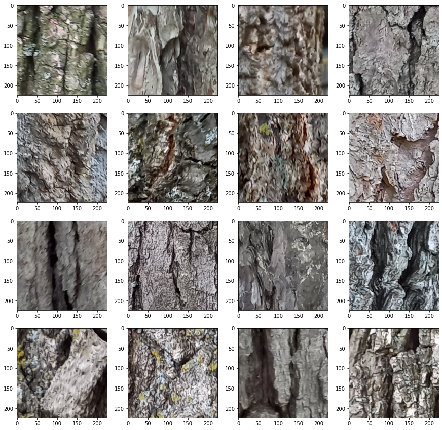
As above, these are all of the accepted bark patches, not just those that have a high confidence. Let’s see what happens when we look at the low-confidence accepted patches.

In [45]:
accept_df_below_65 = confidence_threshold(accept_df, thresh=0.65, below=True)
accept_df_below_65_paths = accept_df_below_65['path'].values.tolist()
sample, paths = new_random_grid(accept_df_below_65_paths)
Generating new sample

Here we see that bias that I was talking about before. Note that when we were looking at the rejected bark, we were looking at patches that were divided by a threshold of 0.85 and were already seeing a lot of patches that could easily be accepted. Here, we are looking at a confidence threshold of 0.65 and are still not seeing many that would definitely be rejected.

The cause of the bias is unknown. I made it a special point of training the usable bark sorter on a roughly even split of acceptable and unacceptable bark. Because this was just a secondary tool for the real project, I haven’t had time to deeply investigate why this might be. I suspect there is some deep information theoretical reason for why this happened, perhaps one that will be painfully obvious to any high schooler once the field is more mature. The important thing now is it’s a quirk of the model that I caught early enough to use.

And what do these patches represent?

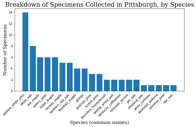
Having seen the images we are working we, it might be a good idea to look at what species we’re actually working with.

In [55]:
specimen_df = pd.read_csv("../specimen_list.csv", index_col=0)
specimen_df
Out[55]:
common_name latin_name family
id
1 norway_maple Acer_platanoides maple
2 norway_maple Acer_platanoides maple
3 norway_maple Acer_platanoides maple
4 red_maple Acer_rubrum maple
5 freeman_maple Acer_x_freemanii maple
75 northern_red_oak Quercus_rubra beech
76 northern_red_oak Quercus_rubra beech
77 white_oak Quercus_alba beech
78 bur_oak Quercus_macrocarpa beech
79 swamp_white_oak Quercus_bicolor beech

79 rows × 3 columns

Okay, I took photos of 79 different trees. It was actually 81, but the GPS signal on the last two was too spotty to match them on the map, and they had to be excluded. How can we break this down?

In [76]:
family_names = specimen_df.family.value_counts()
family_names = family_names.to_dict()
f_names = list(family_names.keys())
f_values = list(family_names.values())

header_font = {'family': 'serif', 'color': 'black', 'size': 20}
axis_font = {'family': 'serif', 'color': 'black', 'size': 15}
plt.rcParams['figure.figsize'] = [10, 5]

plt.bar(range(len(family_names)), f_values, tick_label=f_names)
plt.title("Breakdown of Specimens Collected in Pittsburgh, by Family",
         fontdict=header_font)
plt.xlabel("Family", fontdict=axis_font)
plt.ylabel("Number of Specimens", fontdict=axis_font)
plt.show()

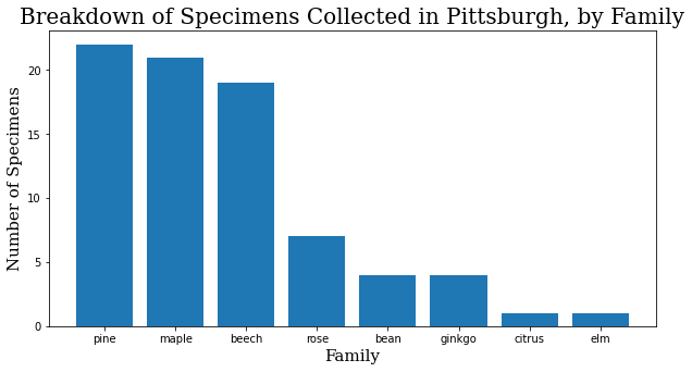
When I started training, it made sense to start training focused on the family level. A family will inherently have at least as many images to work with as a species, and usually many more, and I had the assumption that variation would be smaller within the family. Interestingly enough, at least within this dataset, the difference in the quality of the model at the family and species levels has so far been negligible.

In [80]:
common_names = specimen_df.common_name.value_counts()
common_names = common_names.to_dict()
c_names = list(common_names.keys())
c_values = list(common_names.values())
In [83]:
plt.bar(range(len(common_names)), c_values, tick_label=c_names)
plt.title("Breakdown of Specimens Collected in Pittsburgh, by Species",
         fontdict=header_font)
plt.xlabel("Species (common names)", fontdict=axis_font)
plt.ylabel("Number of Specimens", fontdict=axis_font)
plt.xticks(rotation=45, ha='right')
plt.show()

The Model and Dataset Code

Full code can be found on the GitHub repo, but here are some important parts of the training code. First, because we are using a custom dataset, we need to make a class that will tell the dataloaders what to do. Some of this might need a little bit of explaining.

We have to import some things to make this part of the notebook work. BarkDataset inherits from the Dataset class. To initialize it, we only have to bring a given DataFrame, e.g. accept_df into the class. I’ve shown before that CSVs will let us work with a lot of other data that goes into the support and interpretation of the dataset, but BarkDataset itself only needs two things: the column of all the paths of the images themselves, and the column that defines their labels.

You might be a little confused about the line self.labels = df["factor"].values. The full code converts either the species-level or family-level specimens into a numerical class. For example:

"eastern_white_pine": 0

The label is the 0. When making predictions, we will convert back from this label for clarity to the user, but that isn’t how the model sees it.

After loading the DataFrame, we also define a set of transforms in self.train_transforms. At minimum, this is where we scale images down to 224×224 and normalize them. If you’re wondering, the values for normalization are standard in the field from ImageNet statistics.

In addition to these standard changes, transforms also has a wide variety of transforms that facilitate data augmentation. We can use data augmentation to give us more information from a base dataset; we just need to keep in mind to introduce the kinds of variability that would actually occur in the collection of more data.

You’ll notice two other methods in this class: __len__ and __getitem__. The former just returns the number of items in the DataFrame. The latter is where a single image is actually loaded using Image from the PIL library, and the label is matched from that image’s location in the DataFrame. The transforms are then applied to the image, and we get both the loaded image and its label returned in a dictionary.

In [86]:
import torch
from torch.utils.data import Dataset, DataLoader
from tqdm import tqdm

class BarkDataset(Dataset):
    def __init__(self, df):
        self.df = df
        self.fns = df["path"].values
        self.labels = df["factor"].values

        self.train_transforms = transforms.Compose([
            transforms.ToTensor(),
            transforms.Resize((224, 224)),
            transforms.RandomHorizontalFlip(),
            transforms.RandomRotation(60),
            transforms.ColorJitter(brightness=0.5, contrast=0.5, saturation=0.5, hue=0.5),
            transforms.Normalize(mean=[0.485, 0.456, 0.406],
                                std=[0.229, 0.224, 0.225]),
            ])

    def __len__(self):
        return len(self.df)

    def __getitem__(self, idx):
        row = self.df.iloc[idx]
        image = Image.open(row.path)
        label = self.labels[idx]

        image = self.train_transform(image)

        return {
            "image": image,
            "label": torch.tensor(label, dtype=torch.long)
        }

Next, we’ll look at the model. The model can be expanded in a lot of ways with a class of its own, but at this stage of the project’s development, we are just starting with the pretrained weights and unchanged architecture as provided by timm.

In [ ]:
model = timm.create_model("deit3_base_patch16_224", pretrained=True, num_classes=N_CLASSES)
model.to(device)

criterion = nn.CrossEntropy
optimizer = optim.SGD(model.parameters(), lr=0.001, momentum=0.9)

scheduler = optim.lr_scheduler.CosineAnnealingWarmRestarts(optimizer, T_0=100, T_mult=1,
                                                        eta_min=0.00001, last_epoch=-1)
model, history = training(model, optimizer, criterion, scheduler, device=device, num_epochs=100)
score = testing(test_df, model)

Now, I’ve gone through a lot of iterations of the various components here. Just off the top of my head:

  • I first started using an EfficientNet architecture, but got curious to see how one based on vision transformers would compare, and it wasn’t really a contest.
  • I originally used an Adam optimizer. Training with vanilla SGD proved slower, but also gave more consistent results.
  • I’ve settled on cosine annealing as a learning rate scheduler, but also have intermittent success with CyclicLR and MultiCyclicLR.
  • Most recently, I’ve been wondering if cross-entropy is the right loss metric. I quickly replaced accuracy with ROC because there are multiple, imblanaced classes in the full dataset. I suspect this also has implications for training, but have so far not found a loss metric that works better.

Changing the parameters here is still an active area of my research.

Results

This is a confusion matrix of the results so far. It plots the predicted label against the actual label, and makes it a little easier to see where things are getting mixed up. Ideally, there would only be nonzero values along the diagonal.

In [152]:
#!pip install seaborn
import confusion_stuff
import seaborn as sn

matrix = confusion_stuff.matrix

ind = confusion_stuff.individuals
ind = {k: v for k, v in sorted(ind.items(), key=lambda item: item[1])}
ind_keys = ind.keys()
ind_vals = ind.values()

df_cm = pd.DataFrame(confusion_stuff.matrix)
sn.heatmap(df_cm, cmap="crest")
Out[152]:
<AxesSubplot:>

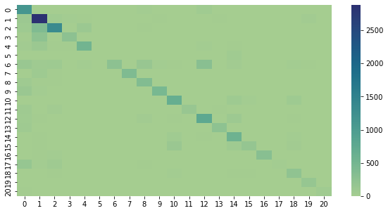
The average ROC for this model across all 21 species is about 0.80. For reference, a 1.0 would be a perfect score, and 0.5 would be random guessing. The graphis is somewhat muddled because there are so many classes, so you can see the scores for individual classes below.

In [153]:
for i, j in zip(ind_keys, ind_vals):
    print(f"{i}: {j}")
common_pear: 0.508
pin_oak: 0.542
red_maple: 0.611
colorado_spruce: 0.69
kentucky_coffeetree: 0.736
chestnut_oak: 0.741
japanese_zelkova: 0.784
northern_red_oak: 0.823
swamp_white_oak: 0.838
scotch_pine: 0.847
sugar_maple: 0.848
callery_pear: 0.857
norway_maple: 0.864
austrian_pine: 0.873
thornless_honeylocust: 0.875
bur_oak: 0.888
eastern_white_pine: 0.888
ginkgo: 0.893
white_oak: 0.912
amur_corktree: 0.921
freeman_maple: 0.922
In [154]:
ind_keys = sorted(list(ind_keys))
ind_vals = sorted(list(ind_vals))
ind_keys.reverse()
ind_vals.reverse()
In [155]:
plt.bar(range(len(ind_keys)), ind_vals, tick_label=ind_keys)
plt.title("ROC of Individual Species in Best Model",
         fontdict=header_font)
plt.xlabel("Species", fontdict=axis_font)
plt.ylabel("ROC", fontdict=axis_font)
plt.xticks(rotation=45, ha='right')
plt.show()

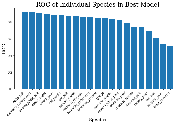
Having plotted these, it’s not hard to see where the model is weak.

Next Steps

I’m still trying new things and learning a lot from this project. Some things on the horizon:

  • Trying one of the larger DeiT models.
  • Ensemble method: training a number of classifiers with a smaller number of classes and having them vote using their confidence scores.
  • Ensemble method: break one large test image into patches, have models vote on each of the patches, and use the majority, the highest confidence, or some other metric as the prediction.
  • Gathering more data, especially expanding to include more species.
  • Weird idea: information theoretical analysis of the tree bark.

Early days!

Deploying PyTorch to an Android Environment

I have some inchoate thoughts about approaches to deployable AI products. Too much of the conversation around AI frames it from the angle of AI-as-a-service, something that a customer makes requests of. This is evidenced by reactions to things like DALL-E 2 being concerned about the possible future of professional artists. A more useful frame of reference is AI-as-an-instrument (AIaaI), i.e. a tool that a user would wield like a pencil. Ideally, it would be something that could amplify arbitrary ideas that a user had. Of course, this would require much more generality than currently trained into models and likely the ability to interface with a number of other APIs.

Exploring a product from this angle will require levering hardware accessible to a normal user, meaning a heavy focus on mobile and edge computing systems. To that end, I’m making a harder pivot to mobile. Fortunately, there is a large and growing body of work being done in the area of mobile deep learning. Before we get started on the really interesting stuff, we have some housekeeping to attend to.

Having done a little work with both, I actually think it will be easier to develop native Android apps instead of using something like React Native. I understand that PyTorch supports both, but the ecosystem for the former seems tighter to me.

Fair warning: because this is covering so much new material, this is going to get long.

GitHub Repo

There is a PyTorch GitHub repo focusing on demos for Android that is worth a look. Today I’ll be going through some of the relevant code in the HelloWorldApp section. Honestly, most of that code. Additionally, I somewhat followed the Quickstart with a HelloWorld Example.

The following is basically notes on things that were confusing or somehow tripped me up in the process of getting HelloWorldApp to run on my phone. If you’re following along and aren’t familiar with Android or Java, I heartily recommend going through the code yourself instead of just downloading and running the repo, especially if you’re most experienced with something like a desktop Python environment. Basically, this picks up from the point of opening Android Studio and starting an empty project.

Gradle Stuff

Gradle is the build tool being used here, and it warrants some attention for anyone coming from the Python landscape or used something like CMake.

Looking at the project structure in Android Studio with the Android view, it’s easy to see that there are two build.gradle files, one for the project and one for the module. For future reference, the Project version is placed in the root folder and wil define behavior for the entire project. A module, being isolated from the broader project, has its own file to define settings that are only relevant to that module.

setttings.gradle

We need to configure this file at the top level. Possibly due to the specifics of my machine, I encountered build errors when starting with the boilerplate file, as follows.

pluginManagement {
    repositories {
        gradlePluginPortal()
        google()
        mavenCentral()
    }
}

dependencyResolutionManagement {
    repositoriesMode.set(RepositoriesMode.FAIL_ON_PROJECT_REPOS)  
    repositories {
        google()
        mavenCentral()
    }
}

rootProject.name = "HelloWorld"
include ':app'

I initially had a look at how to configure a build focusing on settings.gradle and thought that dependencyResolutionManagement had to be removed, but this felt like poor form and raised questions about what would be done in later projects that actually needed this. Fortunately, this is known to happen in the latest version of Android Studio.

The culprit is down to the single setting. FAIL_ON_PROJECT_REPOS. The build fails here because we are setting repositories at the project level. If we comment this line out, we’re golden.

build.gradle (:app)

The project-level build.gradle file is a little more involved, and I think it’s worth going over it in sections. Worth noting that this is written in Groovy, which is a whole thing on its own and beyond the scope of this article.

plugins {
    id 'com.android.application'
}

Here is where we specify plugins. This project in particular just uses the one. com.android.application is used here because the project is an app. For examples of what else might be listed here, library would be com.android.application, or using Kotlin would be org.jetbrains.kotlin.android. There are rich gradle docs going into more detail about the use of plugins.

android {
    compileSdk 32

    defaultConfig {
        applicationId "com.example.helloworld"
        minSdk 28
        targetSdk 31
        versionCode 1
        versionName "1.0"

        testInstrumentationRunner "androidx.test.runner.AndroidJUnitRunner"
    }

    buildTypes {
        release {
            minifyEnabled false
            proguardFiles getDefaultProguardFile('proguard-android-optimize.txt'), 'proguard-rules.pro'
        }
    }

    compileOptions {
        sourceCompatibility JavaVersion.VERSION_1_8
        targetCompatibility JavaVersion.VERSION_1_8
    }  
}

Here is where the specifics of the Android build happen. Looking at defaultConfig, we can see that the name of our app is com.example.helloworld, the earliest Android version that this app can run on is 28, it’s really made for version 31 and compiled against 32, and that it’s version 1.0.

minifyEnabled might seem a little strange. I ran a search and found from this article on shrinking, obfuscating, and optimizing apps. These are things that improve security and shrink the build size. It is disabled by default in Android Studio apps; a developer would need to specify ProGuard rules to enable it, and this is a lightweight example app.

dependencies {
    implementation 'androidx.appcompat:appcompat:1.4.1'
    implementation 'com.google.android.material:material:1.4.0'
    implementation 'androidx.constraintlayout:constraintlayout:2.1.4'
    implementation 'org.pytorch:pytorch_android_lite:1.9.0'
    implementation 'org.pytorch:pytorch_android_torchvision:1.9.0'
    testImplementation 'junit:junit:4.13.2'
    androidTestImplementation 'androidx.test.ext:junit:1.1.3'
    androidTestImplementation 'androidx.test.espresso:espresso-core:3.4.0'
}

The dependencies keyword itself is pretty straightforward, so let’s have a look at what we’re actually using.

Side note: the implementation keyword exists as a way to manage dependencies in chains of libraries and speed up the build time. See Implementation Vs API in Android Gradle plugin 3.0 for more information.

  • AndroidX is the namespace for the Android Jetpack libraries. It’s the replacement for the Android Support Library and used for deployment.
  • AppCompat is a library to make Android apps work across different versions of Android itself.
  • Material Design is the library for Android’s design language.
  • The two PyTorch libraries there provide the actual deep learning functionality that we’ll get to later in this article.
  • testImplementation extends the implementation configuration such that we can use JUnit for tests.

build.gradle (HelloWorld)

With that cleared, we can get into the module-level build.gradle file.

buildscript {
    repositories {
        google()
        jcenter()
    }

    dependencies {
        classpath 'com.android.tools.build:gradle:7.2.0'
    }
}

The buildscript block provides the foundational information for the rest of the build script. Here you can see that we have added

  • google(), which is a shortcut to the Maven repository, and
  • jcenter(), which enables access to a huge number of Java and Android OSS libraries.

Both of these will be downloaded if they are not already installed.

allprojects {
    repositories {
         google()
        jcenter()
    }
}

This might look redundant. allprojects is distinct from buildscript in that the latter is for gradle itself, and the former is for the modules being built by gradle.

task clean(type: Delete) {
    delete rootProject.buildDir
}

Here we just remove the build directory when the app runs. If you want to get a better intuition around tasks, Build Script Basics has a lot of coverage there.

Design Stuff

activity_main.xml

Okay, I’m lying a little bit. Before going over the Java code proper, there is some preliminary work that needs to be done in the design. We need to take a look at activity_main.xml located in the res/values folder, as it is the file that specifies the layout. Android Studio lets you look at the code, the GUI layout, and both side-by-side. Because we are dealing with a relatively simple layout, we’ll just be going over the code in this one.

<?xml version="1.0" encoding="utf-8"?>
<androidx.constraintlayout.widget.ConstraintLayout xmlns:android="http://schemas.android.com/apk/res/android"
 xmlns:app="http://schemas.android.com/apk/res-auto"
 xmlns:tools="http://schemas.android.com/tools"
 android:layout_width="match_parent"
 android:layout_height="match_parent"
 tools:context=".MainActivity">
  ...
</androidx.constraintlayout.widget.ConstraintLayout>

This can be regarded as a bit of boilerplate. For the curious, ConstraintLayout is the parent class of all the design elements that we will be using. It enables the use of the GUI layout editor in Android Studio and avoids nesting of controls.

Being basically a static demonstration, we only need to put two controls inside of this, an ImageView and a TextView. We will explore things like buttons, check boxes, and so on in a later entry.

<ImageView
 android:id="@+id/image"
 android:layout_width="match_parent"
 android:layout_height="match_parent"
 android:scaleType="fitCenter"/>

The image view is where the static image gets displayed. For the sake of simplicity, we will be focusing on the original code and not adding constraints. Those will be part of an upcoming tutorial.

Here, android:id gives the ImageView a name that can be referenced by the activity. layout_width and layout_height are both set to match_parent, indicating that they will be no wider than ConstraintLayout minus its padding. scaleType being set to fitCenter centers the image and matches it to the dimensions of the ImageView. Now, all of this can result in some visual distortions that should be explored when we get to the project that we are ultimately aiming for, but it is being done here to give a consistent presentation for the sake of the example.

<TextView
 android:id="@+id/text"
 android:layout_width="match_parent"
 android:layout_height="wrap_content"
 android:layout_gravity="top"
 android:text="TextView"
 android:textSize="18sp"
 tools:layout_editor_absoluteX="169dp"
 tools:layout_editor_absoluteY="540dp" />

Next is the TextView, which needs a little more explaining. We see here that layout_height is set to wrap_content. This means that, instead of taking up as much space as possible, the TextView only expands enough vertically to contain its values. Setting layout_gravity to top pushes it to the top of the screen without changing the size.

Funnily enough, if you compare this code to the GitHub repo, this is where it starts to get really apparent that I made it a point of going through this myself instead of directly copying the repo. If you don’t change these settings, you’ll run into a warning about android:text being hardcoded instead of using a @string resource, which… Yeah, fair enough, but I don’t want to do a separate section on strings.xml. At any rate, that’s something that Android Studio adds.

Something else specific to Android Studio is the tools namespace, which is used by the layout editor. Seriously, if you remove these two and run this on the phone, it’ll run the same. What’s going on here is that tools is trying to ensure consistency between the XML code and the layout GUI.

Given that the last three attributes deal with layout dimensions, you might be wondering what’s going on with sp and dp. sp stands for scale-independent pixels, and dp stands for density-independent pixels. The functional difference between these is that sp is used for text, which is scaled by user preferences, and dp is used for everything else. Setting textSize to 18sp just makes the text conventionally readable.

Additional Files

Okay, there is some housekeeping that needs to be done. From the repo, you’ll need to copy the files in app/src/main/assets. These are just the test image and the pretrained model. Additionally, you’ll need to copy over ImageNetClasses.java from app/src/main/java/org/pytorch/helloworld, which gives you the labels for the classes in question. This goes right next to MainActivity.java. I would go over it if it were anything more complex than a class containing a string, and it’ll be clear enough on the other side of the main Java material here.

Java Stuff

With that, we are finally ready to get to the meat of the project. The entire focus of the rest of this writeup will be in MainActivity.java.

Imports

First, we’ll have a look at our libraries.

package com.example.helloworld;

This creates the package. These are generally used to avoid name conflicts. It isn’t critical here, but it is a good practice to keep an eye out for.

import androidx.appcompat.app.AppCompatActivity;

import android.os.Bundle;

import android.content.Context;
import android.graphics.Bitmap;
import android.graphics.BitmapFactory;
import android.util.Log;
import android.widget.ImageView;
import android.widget.TextView;

As we’ll see in a moment, AppCompatActivity here is the base class for our MainActivity. This allows us to use newer features on older devices.

Broadly speaking, the android package contains the set of tools and resources that will be used by the app. android.content provides basic data handling on the device itself. android.graphics deals more in things that are drawn to the screen, and will be needed to handle the images. I think it’s clear that android.util‘s use here to handle logging, but it also handles a lot of time, string, and numerical data types. Finally, android.widget handles the UI elements such as our ImageView and TextView.

import org.pytorch.IValue;
import org.pytorch.LiteModuleLoader;
import org.pytorch.Module;
import org.pytorch.Tensor;
import org.pytorch.helloworld.ImageNetClasses;
import org.pytorch.torchvision.TensorImageUtils;
import org.pytorch.MemoryFormat;

org.pytorch is the package containing the deep learning components of the app. Notice on line 5 that we have added the ImageNetClasses file copied from the GitHub repo.

import java.io.File;
import java.io.FileOutputStream;
import java.io.IOException;
import java.io.InputStream;
import java.io.OutputStream;

Finally, we add the java package. java.io just handles the input and output. This might be strange to someone who is only familiar with interpreted languages like Python.

MainActivity

public class MainActivity extends AppCompatActivity {
...
}

This is wrapped around the entirety of our code here. Notice that MainActivity is a class that extends AppCompatActivity. This class is declares MainActivity public, meaning that it is visible to all other classes. It contains only two methods. The first is onCreate(), which initializes the activity. The second is assetFilePath(), which is a helper method that lets us open our test image.

onCreate()

First, we’ll have a look at onCreate() in a number of sections:

@Override
protected void onCreate(Bundle savedInstanceState) {
    super.onCreate(savedInstanceState);
    setContentView(R.layout.activity_main);

    Bitmap bitmap = null;
    Module module = null;

@Override here indicates that we are overriding the method from the parent class, in this case AppCompatActivity.

Bundle savedInstanceState is the state of the application in a bundle, typically dynamic and non-persistent. This plays an important part in the application life cycle, for instance allowing us to navigate away from the app and come back to it with its data intact.

setContentView(R.layout.activity_main is reference to activity_main.xml that we referenced earlier. R is a class that contains the definitions for all the resources used by the package, so we’ll be seeing it peppered throughout the rest of this writeup.

It is worth noting for anyone coming from Python that Java doesn’t do duck typing; every variable needs a type. Personal note: I’ve done enough with Python to know this is a part of the language I’m going to love. bitmap will ultimately be our image, and module will be the pretrained model that we downloaded from the repo. These are being set up this way to provide them access outside of the following try catch statement:

try {
    bitmap = BitmapFactory.decodeStream(getAssets().open("poodle.jpeg"));
    module = LiteModuleLoader.load(assetFilePath(this, "model.pt"));
} catch (IOException e) {
    Log.e("PytorchHelloWorld", "Error reading assets", e);
    finish();
}

ImageView imageView = findViewById(R.id.image);
imageView.setImageBitmap(bitmap);

This statement will fail if either of those files are missing. getAssets() opens the file from the context of the environment, and that stream is decoded by BitmapFactory. LiteModuleLoader() has to call the helper method to open the pretrained model, but we’ll take a look at that in just a moment. I made it a point of looking at the docs, and this doesn’t actually include a counterpart that would be implied by Lite.

Successful completion of the try catch statement then allows the code to call the ImageView and fill it with the bitmap we just opened.

final Tensor inputTensor = TensorImageUtils.bitmapToFloat32Tensor(bitmap,  
TensorImageUtils.TORCHVISION_NORM_MEAN_RGB, TensorImageUtils.TORCHVISION_NORM_STD_RGB,  
 MemoryFormat.CHANNELS_LAST  
);

Here is where the bitmap gets converted into a tensor that can be used by PyTorch. The keyword final here indicates that inputTensor is a constant. TensorImageUtils ultimately wants to turn this into a tensor comprised of 32-bit floating point numbers. The two arguments in the middle are hardcoded lists of floating point values specifying mean and standard deviations for R, G, and B components of a given pixel. This is a convention in machine learning that helps eliminate extreme values when training.

Finally, MemoryFormat.CHANNELS_LAST rearranges the tensor to make the channels last in contrast to a contiguous tensor. A contiguous tensor might have a shape of (3, 224, 244), the 3 indicating one channel for each R, G, and B value, and 224s indicating height and width. Channels last simply moves the 3 to the end to fit with PyTorch’s image representation conventions.

final Tensor outputTensor = module.forward(IValue.from(inputTensor)).toTensor();

There are some moving parts here, but this is where the model tries to predict the image’s class. inputTensor is passed to IValue, short for Interpreter Value. IValue is a Java representation of a TorchScript value. It can be any of a number of supported types, as determined by from(). As we can see here, this one is a Tensor. When the prediction is made, it is also converted to a tensor.

final float[] scores = outputTensor.getDataAsFloatArray();

float maxScore = -Float.MAX_VALUE;
int maxScoreIdx = -1;
for (int i = 0; i < scores.length; i++) {
    if (scores[i] > maxScore) {
        maxScore = scores[i];
    maxScoreIdx = i;
    }
}

scores is an array representing each of the possible classes. The highest score is the model’s prediction for the image’s class. To get that prediction, we loop over that array and set maxScoreIdx to the index where the largest number can be found.

String className = ImageNetClasses.IMAGENET_CLASSES[maxScoreIdx];

TextView textView = findViewById(R.id.text);
textView.setText(className);

className is just the human-readable representation of the prediction, which can be found in the ImageNetClasses file. The TextView is found from its name in the R class, and the name of the prediction is assigned to it.

assetFilePath()

This is a helper method that is used by LiteModuleLoader. Its purpose is to make sure that the image file exists and get its path, or throw an exception if something is wrong with the process.

The first argument here is a Context, the global information about the environment provided by Android. As used by onCreate(), the Context in question is just this, a reference to the current object. For our purposes, assetName is simply the filename of the pretrained model, model.pt.

Unlike the onCreate() method, this uses the throws keyword. This portion indicates that the method might return an IOException if something goes wrong in our file handling process.

public static String assetFilePath(Context context, String assetName) throws IOException {

    ...
}

Let’s move on to the implementation of this method.

    File file = new File(context.getFilesDir(), assetName);
    if (file.exists() && file.length() > 0) {
        return file.getAbsolutePath();
    }

It’s worth outlining the order of operations here. The File class here represents the pathname that we will try to open. context.getFilesDir() gets the absolute path to the directory, and as mentioned before, assetName is the filename of the model we are opening, model.pt.

The if block here just checks that the file exists and is a nonzero length, and will close the method and return the path to be opened by LiteModuleLoader in onCreate() if it’s successful. Simple enough, but what happens if either of these conditions are not met?

        try (InputStream is = context.getAssets().open(assetName)) {
            try (OutputStream os = new FileOutputStream(file)) {
                byte[] buffer = new byte[4 * 1024];
                int read;
                while ((read = is.read(buffer)) != -1) {
                    os.write(buffer, 0, read);
                }
                os.flush();
            }
            return file.getAbsolutePath();
        }

These are nested try-with-resoruces expressions. These statements create their respective InputStream and OutputStream and ensure that they are closed when the statements are completed.

What’s going on here? This creates the model file in the event that one does not already exist or the current one has 0 length. An InputStream using the “model.pt” filename is created, indicating that we are ready to input a stream of bytes to is. Then a FileOutputStream is created so that we will be able to write data to the file “model.pt”. A 4KB byte buffer is created, with each value set to 0. In the while block, the buffer is written to os, and the path to the file is returned.

New Beginnings

I now have a framework for experimenting with PyTorch in a mobile environment. Immediate next steps include actually letting a user make selections of images, using an intent to take new images with the phone’s camera, and doing real-time classification with text displayed in the ImageView itself. Early Days!

Tree Identification with ResNet50 – Quick

This is just a quick update following the same format as the last post, but with some minor modifications. In summary, it has been expanded to include 66 of the species of trees included in the Cleveland Metroparks checklists and has been trained using ResNet50 instead of ResNet34.

In [1]:
%matplotlib inline
%reload_ext autoreload
%autoreload 2
In [2]:
from fastai.vision import *
from fastai.datasets import *
from fastai.widgets import *

from pathlib import Path

import matplotlib.pyplot as plt
import pandas as pd
import numpy as np

Having a handful of these parameters available to be tweaked about here is useful, and it’s a format I’m probably going to stick to for small experiments in notebooks like this.

In [3]:
bs = 16
initial_dims = 224
workers = 2
valid = 0.2
In [4]:
IMG_PATH = Path("data/bark_66_categories")
In [5]:
data = ImageDataBunch.from_folder(IMG_PATH, train=".", valid_pct=valid,
                                 ds_tfms=get_transforms(), bs=bs, size=initial_dims,
                                  num_workers=workers).normalize(imagenet_stats)
In [6]:
data.show_batch(rows=4, figsize=(10, 10))
In [7]:
learn = cnn_learner(data, models.resnet50, metrics=error_rate)

Here, we can already see some modest improvements using a model that has a larger capacity. We’ll be training with the larger images immediately after this one to see just how much more performance we can get out of this model.

In [8]:
learn.fit_one_cycle(4)
epoch train_loss valid_loss error_rate time
0 4.757617 4.026068 0.869828 01:18
1 4.145549 3.616853 0.832759 01:19
2 3.440784 3.219274 0.793103 01:19
3 3.002847 3.121537 0.772414 01:18
In [9]:
learn.lr_find()
0.00% [0/1 00:00<00:00]
epoch train_loss valid_loss error_rate time
30.69% [89/290 00:19<00:43 8.9121]
LR Finder is complete, type {learner_name}.recorder.plot() to see the graph.
In [10]:
learn.recorder.plot()
In [11]:
learn.unfreeze()
learn.fit_one_cycle(4, max_lr=1e-4)
epoch train_loss valid_loss error_rate time
0 3.026054 3.164094 0.773276 01:19
1 3.100843 3.155196 0.770690 01:20
2 2.633893 2.938268 0.725000 01:18
3 2.292624 2.934356 0.718966 01:18
In [12]:
learn.save("cpi-0.0_66-categories_resnet50-1")
In [13]:
data_larger = ImageDataBunch.from_folder(IMG_PATH, train=".", valid_pct=valid,
                                 ds_tfms=get_transforms(), bs=bs, size=initial_dims*2,
                                  num_workers=workers).normalize(imagenet_stats)
In [16]:
learn_larger = cnn_learner(data_larger, models.resnet50, metrics=error_rate)
In [18]:
learn_larger.load("cpi-0.0_66-categories_resnet50-1")
In [19]:
learn_larger.fit_one_cycle(4)
epoch train_loss valid_loss error_rate time
0 3.055164 2.551959 0.679310 01:54
1 2.890265 2.595395 0.670690 01:52
2 2.633454 2.443143 0.643103 01:53
3 2.223217 2.389971 0.634483 01:54
In [20]:
interp = ClassificationInterpretation.from_learner(learn_larger)
In [21]:
interp.plot_confusion_matrix(figsize=(24, 24), dpi=60)

Saving this, because we might be able to use it in the future.

In [22]:
learn.save("cpi-0.0_66-categories_resnet50-2")

Next Steps

So, we can do it. We can double the number of classes and, even though they all have less than 100 images, we can still get modestly successful results. Looking at the error rate above, though, it’s still… Not good. I already mentioned in the last post that some of this is due to the taxonomic nature of the dataset. That is, many of these are in the same genus, and even a human might be likely to get them mixed up.

At this point, a good next step is obvious to me; use more than one label for each category. The model getting conifers mixed up with each other indicates that there is the structure for what a conifer broadly looks like. It just needs to be told that that’s a relevant category. From there, it might be able to offer best guesses.

Witht that target in mind, I will see you soon. Early Days!

Tree Identification – Getting Back on the Saddle

A couple of days ago, I used hws to download a very preliminary dataset. The true aim of this project is to identify some local trees by their bark, but today I’m going to use it as an illustration of the importance of dataset curation and one limitation of automated tools. For instance, web scrapers are dumb. Even if an image is incorrectly tagged by a person or ranked weirdly because of a search algorithm, it can still be downloaded into your raw dataset and needs to be processed by a person.

I noticed early on that, when searching for tree bark, Google returned a lot of accurate results at first, but then very quickly moved on to images that were probably of the same kind of three, but featuring leaves, berries, and picnicking families. A lot had already been downloaded, and I need to get back into the swing of fastai, anyway, so it made sense to see what would happen if I just threw all the data at a model to get a baseline.

To get a sense of the species included in this dataset, I found checklists of the local foliage from the Cleveland Metroparks site, then decided to pare down to just the first page of trees that are common or occasional, and don’t have numerous hybridizations. In all, this yielded about 2,500 images across 31 categories. That is to say, my first run captured less than 100 images for each species, which might produce some workable results if those had just been bark, but was almost certainly going to fail when learning so many different features.

To get some housekeeping out of the way, we use the standard imports.

In [1]:
%matplotlib inline
%reload_ext autoreload
%autoreload 2
In [2]:
from fastai.vision import *
from fastai.datasets import *
from fastai.widgets import *

from pathlib import Path

import matplotlib.pyplot as plt
import pandas as pd
import numpy as np
In [3]:
IMG_PATH = Path("data/images")

Because the dataset in question was just downloaded into folders, we’ll be getting an ImageDataBunch using from_folder. From experience, this is probably going to change to handle pandas DataFrames or CSV annotations as the dataset grows. If you’re following, keep an eye on size, bs, and num_workers. size comes in later because we want to squeeze as much as we can out of this data, and retraining a model on scaled-up images is a clever trick for that. bs and num_workers might have to be tuned down to hardware limitations.

In [4]:
data = ImageDataBunch.from_folder(IMG_PATH, train=".", valid_pct=0.2,
                                 ds_tfms=get_transforms(), bs=16, size=224, num_workers=4).normalize(imagenet_stats)

This next line makes it a bit more apparent that the dataset needs to be curated. show_batch() takes a random sample of images; you might see a lot of bark, and you might not.

In [6]:
data.show_batch(rows=4, figsize=(10, 10))

Pressing ahead, we’re just using ResNet34.

In [7]:
learn = cnn_learner(data, models.resnet34, metrics=error_rate)

Here we see that the results leave a lot to be desired. Error rates on the order of 80% are basically noise.

In [8]:
learn.fit_one_cycle(4)
epoch train_loss valid_loss error_rate time
0 4.448251 3.510020 0.870201 00:20
1 3.843391 3.168392 0.811700 00:20
2 3.177452 2.997584 0.802559 00:20
3 2.746491 2.947996 0.804388 00:20

But! We’re going to save it and try training on slightly larger images, anyway, just for fun.

In [9]:
learn.save("cpi-0.0_ueg-1")
learn.unfreeze()
learn.lr_find()
0.00% [0/1 00:00<00:00]
epoch train_loss valid_loss error_rate time
63.97% [87/136 00:11<00:06 9.3524]
LR Finder is complete, type {learner_name}.recorder.plot() to see the graph.

Intuitively, I can see from this plot that this gradient is going to be way too small to get much better out of this.

In [10]:
learn.recorder.plot()
In [20]:
data_336 = ImageDataBunch.from_folder(IMG_PATH, train=".", valid_pct=0.2,
                                          ds_tfms=get_transforms(), bs=16, size=336, num_workers=1).normalize(imagenet_stats)
In [21]:
learn_336 = cnn_learner(data_336, models.resnet34, metrics=error_rate)
In [ ]:
learn_336.load("cpi-0.0_ueg-1")
In [23]:
learn_336.unfreeze()
learn_336.lr_find()
0.00% [0/1 00:00<00:00]
epoch train_loss valid_loss error_rate time
64.71% [88/136 00:42<00:23 11.7046]
LR Finder is complete, type {learner_name}.recorder.plot() to see the graph.
In [24]:
learn_336.recorder.plot()

And here is why I wanted to highlight this technique. The error rate is down ~10-20% just by using the larger images

In [25]:
learn_336.fit_one_cycle(4, max_lr=1e-5)
epoch train_loss valid_loss error_rate time
0 2.877044 2.116479 0.606947 01:18
1 2.843391 2.076565 0.595978 01:18
2 2.735655 2.080849 0.605119 01:19
3 2.642251 2.076464 0.597806 01:18

Because sometimes difficult to figure out what results mean from just looking at the error rate, and it’s helpful to see exactly what is being miscategorized, let’s take a look at a confusion matrix.

In [26]:
interp = ClassificationInterpretation.from_learner(learn_336)

SURPRISE!

In [27]:
interp.plot_confusion_matrix(figsize=(12,12), dpi=60)
In [28]:
learn_336.save("cpi-0.0_ueg-2")

In spite of the small size of the dataset, the model could actually stand to be a lot worse. We see a nice string of correct classifications along the diagonal. What about the deviations? Comparing some of the most prominent misclassifications, e.g. the strong difficulty in telling pin cherry trees from sweet cherry trees, a given person could understand how a mistake was made.

Alright, this is fun. There are a couple of other tools that will let us take a closer look at what is going wrong here. most_confused() here lets us look at every time one class was confused for the other more than once.

In [37]:
interp.most_confused(2, 10)
Out[37]:
[('pin_cherry_bark', 'sweet_cherry_bark', 6),
 ('red_maple_bark', 'silver_maple_bark', 6),
 ('radford_pear_bark', 'canadian_serviceberry_bark', 5),
 ('black_cherry_bark', 'sweet_cherry_bark', 4),
 ('sweet_cherry_bark', 'black_cherry_bark', 4),
 ('allegheny_serviceberry_bark', 'canadian_serviceberry_bark', 3),
 ('black_maple_bark', 'english_field_maple_bark', 3),
 ('black_maple_bark', 'norway_maple_bark', 3),
 ('black_tupelo_bark', 'silver_maple_bark', 3),
 ('boxelder_bark', 'white_ash_bark', 3),
 ('canadian_serviceberry_bark', 'common_serviceberry_bark', 3),
 ('eastern_redbud_bark', 'american_crabapple_bark', 3),
 ('garden_plum_bark', 'honeylocust_bark', 3),
 ('norway_maple_bark', 'white_ash_bark', 3),
 ('pumpkin_ash_bark', 'white_ash_bark', 3),
 ('red_maple_bark', 'sugar_maple_bark', 3),
 ('silver_maple_bark', 'sugar_maple_bark', 3),
 ('sour_cherry_bark', 'black_cherry_bark', 3),
 ('sour_cherry_bark', 'sweet_cherry_bark', 3),
 ('sugar_maple_bark', 'silver_maple_bark', 3),
 ('white_ash_bark', 'boxelder_bark', 3),
 ('ailanthus_bark', 'black_maple_bark', 2),
 ('ailanthus_bark', 'white_ash_bark', 2),
 ('allegheny_serviceberry_bark', 'common_serviceberry_bark', 2),
 ('black_maple_bark', 'silver_maple_bark', 2),
 ('black_tupelo_bark', 'flowering_dogwood_bark', 2),
 ('black_tupelo_bark', 'horse_chestnut_bark', 2),
 ('black_tupelo_bark', 'sugar_maple_bark', 2),
 ('boxelder_bark', 'norway_maple_bark', 2),
 ('canadian_serviceberry_bark', 'allegheny_serviceberry_bark', 2),
 ('common_serviceberry_bark', 'american_crabapple_bark', 2),
 ('common_serviceberry_bark', 'canadian_serviceberry_bark', 2),
 ('common_serviceberry_bark', 'sour_cherry_bark', 2),
 ('eastern_redbud_bark', 'red_maple_bark', 2),
 ('english_field_maple_bark', 'ailanthus_bark', 2),
 ('english_field_maple_bark', 'eastern_redbud_bark', 2),
 ('english_field_maple_bark', 'garden_plum_bark', 2),
 ('flowering_dogwood_bark', 'radford_pear_bark', 2),
 ('garden_plum_bark', 'american_crabapple_bark', 2),
 ('garden_plum_bark', 'sweet_cherry_bark', 2),
 ('green_ash_bark', 'pumpkin_ash_bark', 2),
 ('green_ash_bark', 'white_ash_bark', 2),
 ('honeylocust_bark', 'black_locust_bark', 2),
 ('honeylocust_bark', 'pin_cherry_bark', 2),
 ('horse_chestnut_bark', 'black_cherry_bark', 2),
 ('northern_catalpa_bark', 'red_horsechestnut_bark', 2),
 ('norway_maple_bark', 'black_maple_bark', 2),
 ('norway_maple_bark', 'sugar_maple_bark', 2),
 ('ohio_buckeye_bark', 'sweet_cherry_bark', 2),
 ('pin_cherry_bark', 'canadian_serviceberry_bark', 2),
 ('pin_cherry_bark', 'sour_cherry_bark', 2),
 ('pumpkin_ash_bark', 'green_ash_bark', 2),
 ('red_horsechestnut_bark', 'horse_chestnut_bark', 2),
 ('red_maple_bark', 'norway_maple_bark', 2),
 ('sour_cherry_bark', 'american_crabapple_bark', 2),
 ('sugar_maple_bark', 'red_maple_bark', 2),
 ('white_ash_bark', 'black_tupelo_bark', 2),
 ('white_ash_bark', 'pumpkin_ash_bark', 2),
 ('yellow_buckeye_bark', 'northern_catalpa_bark', 2)]

Finally, we can use plot_top_losses() to look at some details of extreme outliers. Interestingly, we can see here that the losses were enormous. The model’s confidence in its predictions on all of these are extremely low.

In [40]:
interp.plot_top_losses(9, figsize=(20, 20))

Alright, so a lot of work needs to be done here, but I think we have the groundwork for an interesting, workable project. Some good possibilities for next steps might be:

  • Expand the dataset to include bark from all trees listed.
  • An experiment focusing on trees that the checklist mentioned hybridize easily to compare results.
  • Manually paring down the existing dataset; misclassification aside, we can see from the above that the scraper captured images that simply do not belong in the set.

Early Days!

For the ftagn of it

My first entry going over lesson one was basically a whirlwind tour of how to do image classification. Naturally, a lot of interesting content was left out. Today, I’m just poking at the classification system to see if anything changes.

First, I mentioned in the first post that the model was trained using ResNet-34. If you didn’t have a chance to look at Deep Residual Learning for Image Classification, you might not know that there are different sizes of ResNet models that can be used here of various sizes. I’m going to give them a shot. You have an idea what the code should look like. Not that for my purposes, I’m using the dataset with nine classes.

In [2]:
%reload_ext autoreload
%autoreload 2
%matplotlib inline

from fastai.vision import *
from fastai.metrics import error_rate

bs = 64

# Leaving off most of the infrastructure for making and populating the folders for readability.

path = Path("data/fruit")
classes = ['apples', 'bananas', 'oranges', 'grapes', 'pears', 'pineapples', 'nectarines', 'kiwis', 'plantains']

data = ImageDataBunch.from_folder(path, train=".", valid_pct=0.2,
                                 ds_tfms=get_transforms(), size=224, num_workers=4).normalize(imagenet_stats)

Now for the first bit we are using that is different, training with ResNet50. If it weren’t apparent from the name, it uses 50 layers instead of 34. This theoretically gives it a chance to learn more nuance, but it also introduces the risk of overfitting. We go!

In [3]:
learn = cnn_learner(data, models.resnet50, metrics=error_rate)
learn.fit_one_cycle(4)
Total time: 01:20

epoch train_loss valid_loss error_rate time
0 1.540670 0.397189 0.143713 00:38
1 0.851569 0.252047 0.071856 00:13
2 0.590861 0.260350 0.077844 00:14
3 0.448579 0.258741 0.083832 00:13

Differences? Here’s what jumps out at me:

  • This network took about twice as long to train, which is understandable given that it has many more layers.
  • The training time here is not uniformly distributed.
    • Running the other notebook again revealed that the timing for the equivalent using ResNet-34 also wasn’t uniformly distributed; it was just a fluke. I’m still curious as to why it might change, though.
  • We see a substantial improvement in training loss (~0.65 vs. ~0.41), and slight improvement in validation loss (~0.37 vs. 0.32) and error rate (~0.12 vs. ~0.1).

Okay, not bad. On closer inspection, the ResNet-50 example uses a resolution of 299 instead of 224 for its input images. Additionally, it halved the batch size and used the default number of workers (I am operating under the hypothesis that this is for memory reasons). How do those compare?

In [4]:
data = ImageDataBunch.from_folder(path, train=".", valid_pct=0.2,
                                 ds_tfms=get_transforms(), size=299, bs=bs//2).normalize(imagenet_stats)
learn = cnn_learner(data, models.resnet50, metrics=error_rate)
learn.fit_one_cycle(4)
Total time: 01:51

epoch train_loss valid_loss error_rate time
0 1.252562 0.303597 0.089820 00:42
1 0.704307 0.329760 0.101796 00:23
2 0.469999 0.270663 0.125749 00:23
3 0.361943 0.265046 0.119760 00:23

With the higher resolution images, we still see improvement with the training loss, but also some fluctuations in the validation loss and error rate. Granted, my source ran this four eight cycles and saw a similar fluctuation in the initial four. Easily remedied.

In [5]:
learn.fit_one_cycle(4)
Total time: 01:35

epoch train_loss valid_loss error_rate time
0 0.120617 0.297528 0.107784 00:23
1 0.134901 0.270895 0.077844 00:23
2 0.124303 0.296516 0.101796 00:23
3 0.117052 0.297157 0.113772 00:23

I’m seeing training loss of ~0.12, validation loss of ~0.30, and an error rate of ~0.11. What does all of this mean?

Relationship of Training Loss, Validation Loss, and Error Rate

All of this is very abstract, so I decided to do some searching. Andrej Karpathy has a GitHub page that, among other things, includes tips for the interpretation of these values. Using this as a reference, because our training loss is much smaller than our validation loss, this model is probably overfitting.

In fact, inferring from this advice, we actually want our training loss to be higher than our validation loss. From the looks of it, this learner has been overfitting since epoch 3.

Why?

Simply, loss is an expression of an incorrect prediction; a loss of 0.0 would mean that all of our predictions were correct. Going from Karpathy’s post above, why do we want our training loss to be larger than our validation loss? In that situation, it would mean that our training was stringent enough and our model confident enough that it will perform better than expected when being validated.

Why Don’t You Fix Your Little Problem and Light This Candle?

I recently had the luxury/annoyance of having a short layover in the Hartsfield-Jackson Atlanta International Airport. Having basically not heard of this airport (long story), it was not apparent upon landing that I would be walking for half an hour to get to my next flight, or that I would be waiting among crowds of people from Sweden or Nigeria. Amidst the chaos and strss, I was reminded that the Earth is an immense planet that one person can never completely explore, and that this is true in more ways than one.

You’ll find from reading more of Horseless that I’m a generalist. It is of nothing. Right now, I’m doing the fast.ai course v3, and today I’m following along with lesson 1. Special thanks to Salamander, because frankly, AWS has some work to do on the front end.

It’s been a little while since I’ve used Jupyter notebooks (I’m writing all of this in one right now to get the hang of it again), so I totally forget about the existence of magics. There are tons, but the ones that are relevant to this image classification example are as follows.

We use these magics to reload modules automatically if they have been changed. If that sounds weird, there’s a brief, straighforward example in the docs.

In [1]:
%reload_ext autoreload
%autoreload 2

A lot of magics can also be used in IPython, but this one is specific to Jupyter notebooks. This just allows us to display matplotlib graphs in the notebook itself.

In [2]:
%matplotlib inline

Naturally, we have a couple of library imports. I’ve gotten into the habit of at least peaking at the docs whenever I run into a new library, especially when we’re importing everything. The documentation for fastai.vision is actually pretty short and readable.

In [3]:
from fastai.vision import *
from fastai.metrics import error_rate

bs just sets the batch size.

In [4]:
bs = 64

Deception!

This blog entry isn’t completely following the pets example. I’m also looking at an image download guide that I guess is from the next lesson. For this, I wanted to build a classifier of fruit using scraped images and see how well it scales with the number of categories and such.

Well, that’s what’s going on here. Basically, we make a Path object to hold all of our different classes. Classes here are assigned new folders; this snippet will make a new folder for each class if it doesn’t already exist. It looks like overkill here, and even the original tutorial in the image download tutorial only had three different classes for bears, but part of my exploration of lesson one will be looking at how the model responds to different numbers of classes.

In [5]:
path = Path("data/fruit1")

folders = ['apples','bananas', 'oranges']
for folder in folders:
    dest = path/folder
    dest.mkdir(parents=True, exist_ok=True)

If you don’t recognize ls as a CLI command, this just gets a list of all the non-hidden files and folders in the current working directory. I’ve probably run this notebook half a dozen times, so my original view of it was pretty thoroughly populated. You’ll see in a minute why having multiple folders for each of these runs was a good idea.

In [15]:
path.ls()
Out[15]:
[PosixPath('data/fruit1/apples'),
 PosixPath('data/fruit1/bananas'),
 PosixPath('data/fruit1/urls_apples.txt'),
 PosixPath('data/fruit1/.ipynb_checkpoints'),
 PosixPath('data/fruit1/oranges'),
 PosixPath('data/fruit1/urls_oranges.txt'),
 PosixPath('data/fruit1/urls_bananas.txt')]

This next bit is where we get into some annoying stuff in the tutorial that I want to come back and fix later. We need data to many anything happen here, and a quick way to get data for our purposes here is to run a search on Google Images for, let’s say, apples. The tutorial wants us to save those URLs, and to do that, we need a bit of code:

urls = Array.from(document.querySelectorAll('.rg_di .rg_meta')).map(el=>JSON.parse(el.textContent).ou);
window.open('data:text/csv;charset=utf-8,' + escape(urls.join('\n')));

It’s JavaScript, my old nemesis. The tutorial just says that this is to be entered into the browser’s ‘Console’, and suggests that Ctrl + Shift + J brings this up for Firefox. Maybe I spent too much time messing with the settings or something, because that brought up a (for this) worthless display console. For Firefox, I needed to go to Tools -> Web Developer -> Web Console to enter this code, which I only later learned was Shift + Ctrl + K.

Anyway, this needs to be repeated for each class. It’s automatish. The video links to a different set of tips for downloading images using a tool called googleimagesdownload that I had a chance to use once, but getting that working involved enough installation, weird complications, and documentation that would be better suited for another entry. We’re not fighting Raktabija today.

This snippet is straightforward enough. Go through each of the classes and use download_images to download up to 200 images for each one. Yes, I’m leaving those prints in. Full disclosure, I was looking at three different examples and was way more confused than I should have been for about 20 minutes. Those things are heroes.

That said, funny story, true story. For some reason, my urls_apples.txt file has 200 links, twice as many as the others here. I don’t know why. Maybe I scrolled down farther in the Google Images results than the others and the code included the extra ones that were dynamically loaded on the page. Maybe I was playing with a different piece of code when I was first doing this at 0230 and forgot about it. Maybe I’m a crazy man on the Internet who doens’t know what he’s talking about because it works on your machine.

The thing is, this isn’t trivial! My original run had twice as many examples of apples to draw from as anything else, which could easily change its performance. My point is, be careful. There’s a lot of work to do here.

In [16]:
for folder in folders:
    file = "urls_" + folder + ".txt"
    print(file)
    print(folder)
    print(path)
    download_images(path/file, path/folder, max_pics = 100)
urls_apples.txt
apples
data/fruit1
100.00% [100/100 00:14<00:00]
Error https://www.washingtonpost.com/resizer/Q2AWXkiQTsKIXHT_91kZWGIFMRY=/1484x0/arc-anglerfish-washpost-prod-washpost.s3.amazonaws.com/public/YCFJ6ZPYZQ2O5ALQ773U5BA7GU.jpg HTTPSConnectionPool(host='www.washingtonpost.com', port=443): Read timed out. (read timeout=4)
urls_bananas.txt
bananas
data/fruit1
100.00% [100/100 00:05<00:00]
Error https://www.kroger.com/product/images/xlarge/front/0000000004237 HTTPSConnectionPool(host='www.kroger.com', port=443): Read timed out. (read timeout=4)
urls_oranges.txt
oranges
data/fruit1
100.00% [100/100 00:03<00:00]

verify_images is used to do a bit of preliminary cleanup. Here, it will delete images that are broken and resize them so that each one is no larger than 500 pixels on a side. The documentation promises that the original ratios are preserved, so we should be good to go.

In [17]:
for f in folders:
    print(f)
    verify_images(path/f, delete=True, max_size=500)
apples
100.00% [97/97 00:03<00:00]
cannot identify image file <_io.BufferedReader name='data/fruit1/apples/00000096.jpg'>
cannot identify image file <_io.BufferedReader name='data/fruit1/apples/00000050.png'>
cannot identify image file <_io.BufferedReader name='data/fruit1/apples/00000088.jpg'>
cannot identify image file <_io.BufferedReader name='data/fruit1/apples/00000068.png'>
cannot identify image file <_io.BufferedReader name='data/fruit1/apples/00000031.jpg'>
cannot identify image file <_io.BufferedReader name='data/fruit1/apples/00000015.jpg'>
cannot identify image file <_io.BufferedReader name='data/fruit1/apples/00000055.jpg'>
bananas
100.00% [98/98 00:02<00:00]
cannot identify image file <_io.BufferedReader name='data/fruit1/bananas/00000015.jpg'>
cannot identify image file <_io.BufferedReader name='data/fruit1/bananas/00000061.jpg'>
oranges
100.00% [100/100 00:02<00:00]
cannot identify image file <_io.BufferedReader name='data/fruit1/oranges/00000009.jpg'>
cannot identify image file <_io.BufferedReader name='data/fruit1/oranges/00000011.png'>
cannot identify image file <_io.BufferedReader name='data/fruit1/oranges/00000048.jpg'>
/home/ubuntu/anaconda3/lib/python3.7/site-packages/PIL/Image.py:965: UserWarning: Palette images with Transparency   expressed in bytes should be converted to RGBA images
  ' expressed in bytes should be converted ' +
cannot identify image file <_io.BufferedReader name='data/fruit1/oranges/00000078.jpg'>
cannot identify image file <_io.BufferedReader name='data/fruit1/oranges/00000090.jpg'>
cannot identify image file <_io.BufferedReader name='data/fruit1/oranges/00000092.jpg'>

Seriously, that many?! I’m going to be using this thing all the time.

Get on with it!

We set the random seed for reproducibility. I remember this being wonky when I did this in Keras, but we’ll roll with it for now.

I do recommend having a look at the documentation for ImageDataBunch. What’s going on here? Images from the specified folder are collected. valid_pct holds out 20% of the images for validation (0.2 is provided as a default if you leave it out). ds_tfms=get_transforms() is gives us a set of default data augmentation features like flipping the images on the axis.

In [6]:
np.random.seed(42)
data = ImageDataBunch.from_folder(path, train=".", valid_pct=0.2,
                                 ds_tfms=get_transforms(), size=224, num_workers=4).normalize(imagenet_stats)

Just a quick peek to see where we are that we have the right classes and see if anything obvious weird happened with our images.

In [19]:
data.classes
Out[19]:
['apples', 'bananas', 'oranges']
In [20]:
data.show_batch(rows=3, figsize=(7,8))

This is the juicy part (but it does look a bit light if you’re familiar with Keras). Here we put our dataset into a convolutional neural network. The model that we’re using here is the pretrained ResNet-34, a midsized residual network. If you’re into the background, I recommend familiarizing yourself with the paper Deep Residual Learning for Image Recognition, which I’ll be talking about in a later post. There is a lot to unpack here.

In [7]:
learn = cnn_learner(data, models.resnet34, metrics=error_rate)

Now, we just train the learner for four epochs.

In [71]:
learn.fit_one_cycle(4)
Total time: 00:16

epoch train_loss valid_loss error_rate time
0 1.376529 0.612187 0.232143 00:04
1 0.873382 0.127812 0.000000 00:04
2 0.622132 0.040325 0.000000 00:04
3 0.467340 0.029021 0.000000 00:03

Now we save these weights, because we’re about to see what happens when we train the entire model. Up until now, we’ve only trained a portion of the network, but unfreeze() will allow us to train on all of the weights. lr_find() will train with a number of different learnings rates.

In [72]:
learn.save('fruit-1')
learn.unfreeze()
learn.fit_one_cycle(1)
Total time: 00:04

epoch train_loss valid_loss error_rate time
0 0.097448 0.104915 0.053571 00:04
LR Finder is complete, type {learner_name}.recorder.plot() to see the graph.

This bit of code will graph the results of lr_find().

In [74]:
learn.lr_find()
learn.recorder.plot()
LR Finder is complete, type {learner_name}.recorder.plot() to see the graph.

We run fit one cycle, using values from the graph where the loss starts to be minimized.

In [75]:
learn.fit_one_cycle(3, max_lr=slice(3e-4, 3e-3))
Total time: 00:13

epoch train_loss valid_loss error_rate time
0 0.068045 0.043532 0.017857 00:04
1 0.059558 0.174751 0.053571 00:04
2 0.046345 0.114111 0.035714 00:04

… Okay! The training loss and error rate are decreasing, but the validation loss is on the rise. The network might be overfitting a bit here, but we shall see how it performs. I’m not especially confident that we have a total improvement here, so we will save this as a separate model.

In [76]:
learn.save('fruit-2')

ClassificationInterpretation can take a Learner and plot a confusion matrix, a grid indicating what the model predicted a given image was versus what it actually was. Because of the way the graphic is set up, it is visually easy to see that a model has achieved a low error rate by looking at its characteristic solid diagonal line with maybe a few missed cases here and there.

In [79]:
interp = ClassificationInterpretation.from_learner(learn)
interp.plot_confusion_matrix()

Expanded number of classes.

Not bad, but we can try something a bit more complicated. Let’s repeat the above steps using nine categories instead of three.

In [8]:
path = Path("data/fruit")

folders = ['apples', 'bananas', 'oranges', 'grapes', 'pears', 'pineapples', 'nectarines', 'kiwis', 'plantains']

for folder in folders:
    dest = path/folder
    dest.mkdir(parents=True, exist_ok=True)
In [50]:
path.ls()
Out[50]:
[PosixPath('data/fruit/apples'),
 PosixPath('data/fruit/urls_kiwis.txt'),
 PosixPath('data/fruit/bananas'),
 PosixPath('data/fruit/grapes'),
 PosixPath('data/fruit/urls_plantains.txt'),
 PosixPath('data/fruit/urls_pineapples.txt'),
 PosixPath('data/fruit/urls_apples.txt'),
 PosixPath('data/fruit/models'),
 PosixPath('data/fruit/kiwis'),
 PosixPath('data/fruit/.ipynb_checkpoints'),
 PosixPath('data/fruit/oranges'),
 PosixPath('data/fruit/urls_pears.txt'),
 PosixPath('data/fruit/nectarines'),
 PosixPath('data/fruit/urls_nectarines.txt'),
 PosixPath('data/fruit/urls_oranges.txt'),
 PosixPath('data/fruit/urls_grapes.txt'),
 PosixPath('data/fruit/pears'),
 PosixPath('data/fruit/plantains'),
 PosixPath('data/fruit/pineapples'),
 PosixPath('data/fruit/urls_bananas.txt')]
In [51]:
for folder in folders:
    file = "urls_" + folder + ".txt"
    download_images(path/file, path/folder, max_pics = 200)
100.00% [100/100 00:13<00:00]
Error https://www.washingtonpost.com/resizer/Q2AWXkiQTsKIXHT_91kZWGIFMRY=/1484x0/arc-anglerfish-washpost-prod-washpost.s3.amazonaws.com/public/YCFJ6ZPYZQ2O5ALQ773U5BA7GU.jpg HTTPSConnectionPool(host='www.washingtonpost.com', port=443): Read timed out. (read timeout=4)
100.00% [100/100 00:05<00:00]
Error https://www.kroger.com/product/images/xlarge/front/0000000004237 HTTPSConnectionPool(host='www.kroger.com', port=443): Read timed out. (read timeout=4)
100.00% [100/100 00:03<00:00]
100.00% [100/100 00:06<00:00]
Error https://www.washingtonpost.com/resizer/c8KGxTwvfOVZuG4hd_vlgUIHdwU=/1484x0/arc-anglerfish-washpost-prod-washpost.s3.amazonaws.com/public/XXA47NWIRII6NC7OKTUAB3ZKMM.jpg HTTPSConnectionPool(host='www.washingtonpost.com', port=443): Read timed out. (read timeout=4)
Error https://www.kroger.com/product/images/xlarge/front/0000000094022 HTTPSConnectionPool(host='www.kroger.com', port=443): Read timed out. (read timeout=4)
Error https://www.washingtonpost.com/rf/image_982w/2010-2019/WashingtonPost/2017/10/11/Food/Images/SheetPanSausageDinner-1733.jpg HTTPSConnectionPool(host='www.washingtonpost.com', port=443): Read timed out. (read timeout=4)
100.00% [100/100 00:03<00:00]
100.00% [100/100 00:04<00:00]
Error https://cdn.teachercreated.com/20180323/covers/900sqp/2156.png HTTPSConnectionPool(host='cdn.teachercreated.com', port=443): Max retries exceeded with url: /20180323/covers/900sqp/2156.png (Caused by SSLError(SSLError("bad handshake: Error([('SSL routines', 'tls_process_server_certificate', 'certificate verify failed')])")))
100.00% [100/100 00:09<00:00]
100.00% [100/100 00:04<00:00]
100.00% [100/100 00:04<00:00]
Error https://blog.heinens.com/wp-content/uploads/2016/03/Plantains_Blog-Feature.jpg HTTPSConnectionPool(host='blog.heinens.com', port=443): Max retries exceeded with url: /wp-content/uploads/2016/03/Plantains_Blog-Feature.jpg (Caused by SSLError(SSLError("bad handshake: Error([('SSL routines', 'tls_process_server_certificate', 'certificate verify failed')])")))
Error https://www.washingtonpost.com/resizer/dJ0Bg2LQrSAaSo6UlPbKm6J4SJ8=/1484x0/arc-anglerfish-washpost-prod-washpost.s3.amazonaws.com/public/Y6C5GNMXEA2XJL5TQXJTF6DXPQ.jpg HTTPSConnectionPool(host='www.washingtonpost.com', port=443): Read timed out. (read timeout=4)
In [52]:
for f in folders:
    print(f)
    verify_images(path/f, delete=True, max_size=500)
apples
100.00% [97/97 00:03<00:00]
cannot identify image file <_io.BufferedReader name='data/fruit/apples/00000050.png'>
cannot identify image file <_io.BufferedReader name='data/fruit/apples/00000096.jpg'>
cannot identify image file <_io.BufferedReader name='data/fruit/apples/00000088.jpg'>
cannot identify image file <_io.BufferedReader name='data/fruit/apples/00000068.png'>
cannot identify image file <_io.BufferedReader name='data/fruit/apples/00000031.jpg'>
cannot identify image file <_io.BufferedReader name='data/fruit/apples/00000015.jpg'>
cannot identify image file <_io.BufferedReader name='data/fruit/apples/00000055.jpg'>
bananas
100.00% [98/98 00:02<00:00]
cannot identify image file <_io.BufferedReader name='data/fruit/bananas/00000015.jpg'>
cannot identify image file <_io.BufferedReader name='data/fruit/bananas/00000061.jpg'>
oranges
100.00% [100/100 00:02<00:00]
cannot identify image file <_io.BufferedReader name='data/fruit/oranges/00000009.jpg'>
cannot identify image file <_io.BufferedReader name='data/fruit/oranges/00000011.png'>
cannot identify image file <_io.BufferedReader name='data/fruit/oranges/00000048.jpg'>
/home/ubuntu/anaconda3/lib/python3.7/site-packages/PIL/Image.py:965: UserWarning: Palette images with Transparency   expressed in bytes should be converted to RGBA images
  ' expressed in bytes should be converted ' +
cannot identify image file <_io.BufferedReader name='data/fruit/oranges/00000078.jpg'>
cannot identify image file <_io.BufferedReader name='data/fruit/oranges/00000090.jpg'>
cannot identify image file <_io.BufferedReader name='data/fruit/oranges/00000092.jpg'>
grapes
100.00% [97/97 00:02<00:00]
cannot identify image file <_io.BufferedReader name='data/fruit/grapes/00000022.png'>
cannot identify image file <_io.BufferedReader name='data/fruit/grapes/00000097.jpeg'>
cannot identify image file <_io.BufferedReader name='data/fruit/grapes/00000027.jpg'>
cannot identify image file <_io.BufferedReader name='data/fruit/grapes/00000092.png'>
/home/ubuntu/anaconda3/lib/python3.7/site-packages/PIL/Image.py:965: UserWarning: Palette images with Transparency   expressed in bytes should be converted to RGBA images
  ' expressed in bytes should be converted ' +
pears
100.00% [100/100 00:03<00:00]
cannot identify image file <_io.BufferedReader name='data/fruit/pears/00000045.png'>
cannot identify image file <_io.BufferedReader name='data/fruit/pears/00000058.jpg'>
cannot identify image file <_io.BufferedReader name='data/fruit/pears/00000084.png'>
/home/ubuntu/anaconda3/lib/python3.7/site-packages/PIL/Image.py:965: UserWarning: Palette images with Transparency   expressed in bytes should be converted to RGBA images
  ' expressed in bytes should be converted ' +
/home/ubuntu/anaconda3/lib/python3.7/site-packages/PIL/Image.py:965: UserWarning: Palette images with Transparency   expressed in bytes should be converted to RGBA images
  ' expressed in bytes should be converted ' +
cannot identify image file <_io.BufferedReader name='data/fruit/pears/00000068.jpg'>
cannot identify image file <_io.BufferedReader name='data/fruit/pears/00000029.jpg'>
cannot identify image file <_io.BufferedReader name='data/fruit/pears/00000031.png'>
/home/ubuntu/anaconda3/lib/python3.7/site-packages/PIL/Image.py:965: UserWarning: Palette images with Transparency   expressed in bytes should be converted to RGBA images
  ' expressed in bytes should be converted ' +
cannot identify image file <_io.BufferedReader name='data/fruit/pears/00000081.jpg'>
pineapples
100.00% [99/99 00:04<00:00]
cannot identify image file <_io.BufferedReader name='data/fruit/pineapples/00000048.jpg'>
cannot identify image file <_io.BufferedReader name='data/fruit/pineapples/00000032.jpg'>
cannot identify image file <_io.BufferedReader name='data/fruit/pineapples/00000012.jpg'>
/home/ubuntu/anaconda3/lib/python3.7/site-packages/PIL/Image.py:1018: UserWarning: Couldn't allocate palette entry for transparency
  warnings.warn("Couldn't allocate palette entry " +
cannot identify image file <_io.BufferedReader name='data/fruit/pineapples/00000034.jpg'>
nectarines
100.00% [100/100 00:02<00:00]
cannot identify image file <_io.BufferedReader name='data/fruit/nectarines/00000011.png'>
cannot identify image file <_io.BufferedReader name='data/fruit/nectarines/00000051.png'>
cannot identify image file <_io.BufferedReader name='data/fruit/nectarines/00000088.jpg'>
cannot identify image file <_io.BufferedReader name='data/fruit/nectarines/00000005.jpg'>
cannot identify image file <_io.BufferedReader name='data/fruit/nectarines/00000062.jpg'>
cannot identify image file <_io.BufferedReader name='data/fruit/nectarines/00000098.jpg'>
cannot identify image file <_io.BufferedReader name='data/fruit/nectarines/00000095.jpg'>
cannot identify image file <_io.BufferedReader name='data/fruit/nectarines/00000080.jpg'>
cannot identify image file <_io.BufferedReader name='data/fruit/nectarines/00000038.jpg'>
kiwis
100.00% [98/98 00:02<00:00]
cannot identify image file <_io.BufferedReader name='data/fruit/kiwis/00000084.png'>
cannot identify image file <_io.BufferedReader name='data/fruit/kiwis/00000078.jpg'>
cannot identify image file <_io.BufferedReader name='data/fruit/kiwis/00000056.jpg'>
cannot identify image file <_io.BufferedReader name='data/fruit/kiwis/00000068.jpg'>
cannot identify image file <_io.BufferedReader name='data/fruit/kiwis/00000075.jpg'>
plantains
100.00% [97/97 00:02<00:00]
cannot identify image file <_io.BufferedReader name='data/fruit/plantains/00000052.jpg'>
local variable 'photoshop' referenced before assignment
cannot identify image file <_io.BufferedReader name='data/fruit/plantains/00000083.jpg'>
cannot identify image file <_io.BufferedReader name='data/fruit/plantains/00000044.jpg'>
In [12]:
data2 = ImageDataBunch.from_folder(path, train=".", valid_pct=0.2,
                                 ds_tfms=get_transforms(), size=224, num_workers=4).normalize(imagenet_stats)
In [13]:
learn2 = cnn_learner(data2, models.resnet34, metrics=error_rate)
In [14]:
learn2.fit_one_cycle(4)
Total time: 00:31

epoch train_loss valid_loss error_rate time
0 2.030864 0.831149 0.221557 00:08
1 1.239848 0.415597 0.119760 00:07
2 0.863067 0.377215 0.119760 00:07
3 0.657382 0.371677 0.113772 00:07
In [93]:
learn2.save('large-fruit-1')
interp2 = ClassificationInterpretation.from_learner(learn2)
interp2.plot_confusion_matrix()

Much more interesting. Even without the unfreezing and optimization, we see decent results with a larger number of categories. Additionally, where you see some more prominent spots of confusing, it is worth actually thinking about what might be tripping the model up. Depending on the image, a nectarine can sort of look like an apple. Being from the US, plantains to me are basically bananas that are always green.

You’ll notice that we didn’t do that unfreeze-and-optimize strategy from before, so let’s see what that looks like.

In [94]:
learn2.unfreeze()
learn2.fit_one_cycle(1)
Total time: 00:10

epoch train_loss valid_loss error_rate time
0 0.366309 0.297740 0.113772 00:10
In [95]:
learn2.lr_find()
learn2.recorder.plot()
LR Finder is complete, type {learner_name}.recorder.plot() to see the graph.

Well, that sure looks like a different loss graph.

In [97]:
learn2.save('large-fruit-2')
In [106]:
learn2.load('large-fruit-2')
learn2.fit_one_cycle(3, max_lr=slice(1e-5, 1e-3))
Total time: 00:30

epoch train_loss valid_loss error_rate time
0 0.226404 0.285319 0.101796 00:10
1 0.167561 0.261312 0.083832 00:10
2 0.128132 0.265344 0.071856 00:09
In [107]:
interp2 = ClassificationInterpretation.from_learner(learn2)
interp2.plot_confusion_matrix()

Training loss has been cut significantly, but validation loss and error rates are holding steady. There is a lot of unpacking to be done. Early days!